On Singular Value Decomposition and Its Use in Recommendation Systems

Since the dawn of time, human beings have asked some fundamental questions: who are we? why are we here? is there life after death? Unable to answer any of these, in this post we will learn what Singular Value decomposition is and how it can be used in recommender systems. SVD (Singular Value Decomposition) is one of the most beautiful equation of mathematics and a highlight of linear algebra. You can think of it as a data reduction tool. It's an algorithm that you need to learn if you want to make money using linear algebra. In this post I will only assume you can calculate eignevalues and eigenvectors :) You can skip to the second part of this discussion to avoid delving too deeply into the mathematical details and instead focus on understanding the more practical aspects related to recommendations - the applied side of the mathematics.

1. Understanding SVD

I will start by presenting to you the formula for singular value decomposition. Given an $m$ -by- $n$ matrix $A$ , the singular value decomposition (SVD) can be expressed as:

$A = U \Sigma V^{T} \tag{1}$

Two important aspects of formula $(1)$ are:

The dimensions of the factors: $U \in \mathbb{R}^{m \times m}$ , $\Sigma \in \mathbb{R}^{m \times n}$ , $V \in \mathbb{R}^{n \times n}$ .
$U$ and $V$ are orthogonal matrices, while $\Sigma$ is a diagonal matrix.

This decomposition structure is similar to eigendecomposition, and formula $(1)$ can be derived by performing eigendecompositions on $A^{T}A$ and $AA^{T}$ , which are symmetric matrices.

For eigendecomposition, when you see $A = Q \Lambda Q^{-1}$ , $Q$ represents the matrix of eigenvectors of $A$ , and $\Lambda$ is the matrix with the ordered eigenvalues of $A$ .

Calculating $A^{T}A$ assuming formula $(1)$ :

$A^{T}A = (U \Sigma V^{T})^{T}(U \Sigma V^{T}) = (V \Sigma U^{T})(U \Sigma V^{T}) = V \Sigma^2 V^{T} \tag{2}$

Substituting $\Sigma^2$ with $\Lambda$ , equation $(2)$ becomes:

$A^{T}A = V \Sigma^2 V^{T} = V \Lambda V^{T} = V \Lambda V^{-1} \tag{3}$

Since $V$ is an orthogonal matrix, $V^{T} = V^{-1}$ . The orthogonality of $U$ and $V$ ensures that the transformation preserves the geometry of the original data as much as possible while reducing its dimensionality, which is crucial for applications like dimensionality reduction and data compression. You can now compare equation $(3)$ with $Q \Lambda Q^{-1}$ to see how eigencompostion is used here.

Intuitively speaking, because matrix $A$ is not necessarily square, we calculate $A^{T}A$ to make it square, then perform the familiar eigendecomposition. Note that we have orthogonal eigenvectors in this case because $A^{T}A$ is a symmetric matrix. Let's continue with our exploration of the SVD formula by turning our attention from matrix $V$ ---a factor of eigendecomposition on $A^{T}A$ ---to the matrix $U$ .

Much like we understood $V$ as a factor of eigendecomposition, $U$ can be seen as a factor of eigendecomposition, this time on the matrix $AA^T$ . Concretly,

$AA^{T} = (U \Sigma V^{T})(U \Sigma V^{T})^{T} = (U \Sigma V^{T})(V \Sigma U^{T}) = U \Sigma^2 U^T \tag{4}$

Notice the parallel between (2) and (4). It's not difficult to see that, by symmetry, $U$ is also going to be an orthogonal matrix containing the eigenvectors of $AA^T$ . The most important difference between $U$ and $V$ concerns dimensionality: while $U$ is a $m$ -by- $m$ matrix, V is an $n$ -by- $n$ . This disparity originates from the fact that $A$ itself is a rectangular matrix, meaning that the dimensions of $AA^{T}$ and $A^{T}A$ are also different. Another point that requires clarification pertains to $\Sigma$ . Earlier, we made a substitution of $\Sigma^2$ for $\Lambda$ . This tells us that $\Sigma$ contains the square roots of the eigenvalues of $A^{T}A$ and $AA^T$ , which, it is important to note, has identical non-zero eigenvalues. If this point brings confusion, let me summarise the SVD below:

$U$ and $V^{T}$ are called left singular and right singular vectors.
$\Sigma$ contains what are called Sigular values.
Since $A$ is rectangular, we use $A^{T}A$ and $AA^T$ , which are square, to calculate the eigendecomposition.
Solving this eigen decompostition we will get $U$ , $V^{T}$ & $\Sigma$ - which is just the square root of eigenvalues of $A^{T}A$ and $AA^T$
Even though $A^{T}A$ and $AA^T$ have different shapes, $\Sigma$ for both will contain same non-zero singularvalues. The one with larger shape will just have extra 0 as singularvalues

Let's conclude this section with the formula for singular value decomposition:

$A = U \Sigma V^{T}$

Hopefully, now it is clear what $U$ , $\Sigma$ , and $V$ are. Singular value decomposition can intuitively be thought of as a square root version of eigendecomposition, since essentially $U$ and $V$ are all derivatives that come from the "square" of a matrix, the two transpose multiples. This intuition also aligns with the fact that $\Sigma$ is a diagonal matrix containing the square roots of eigenvalues of the transpose products. Another beautiful representation of SVD is to learn that you can also think of the SVD in this form:

$A = \sigma_1 u_1 v_1^{T} + \sigma_2 u_2 v_2^{T} + \sigma_3 u_3 v_3^{T} + \sigma_3 u_3 v_3^{T} + ...$

and $\sigma_1 >= \sigma_2 >= \sigma_3 >= ...$

Here's the interesting part, even if you include in first $r$ entries from this equation,for a reasonable $r$ , you will be able approximate the matrix $A$ . This came from Eckart–Young theorem and is the basis for data reduction.

2. SVD for recommendation (Dense matrix)

With these in mind, let's get ready to build the recommendation model. Suppose you are large drug company. The organic way your drug gets bought is only if there really is no alternative, which isn't always the case. Therefore you must start promotional activities to the doctors, hoping that they will remember the drug's properties and then prescribe yours when the time comes!

So now you start your marketing activities and promotion on all of the available channels to you for e.g. it could be a person visiting doctor for the promotion, someone calling the doctors, you asking some other third-party agencies to do this on your behalf where you are unreachable or even conducting seminars. The possibilities will depend on your creativity. To make things simple let us just name activities of types as channels and let's say you have n channels. You have identified your doctors for whom you would like these activities to occur and have shortlisted m doctors.

Hypothetically, suppose you also happen to know how a doctor rates each of your channel out of 10. For example, if a doctor really likes channel 1 so he rates it 10 and dislikes channel 10 so he rates it 1. Ideally, you as a drug company will not have this rating but can always use different proxies and come up with one that is synthesize your rating using data. Again, it depends on your creativity.

So let me define a function that can create a doctor ratings matrix for me in python.

def doctor_ratings_matrix(num_users, num_items):
    data = []
    for i in range(num_users):
        user = [np.random.uniform() for _ in range(num_items)]
        data.append(user)
    mat = pd.DataFrame(data)
    mat.index = ["Doctor " + str(i) for i in range(num_users)]
    mat.columns = ["Channel " + str(i) for i in range(num_items)]
    return mat

With this background, after your first round of promotional activity you'll have a rectangular matrix like this:

A = doctor_ratings_matrix(5, 5)
A

| | Channel 0 | Channel 1 | Channel 2 | Channel 3 | Channel 4 | | Doctor 0 | 0.543405 | 0.278369 | 0.424518 | 0.844776 | 0.00471886 | | Doctor 1 | 0.121569 | 0.670749 | 0.825853 | 0.136707 | 0.575093 | | Doctor 2 | 0.891322 | 0.209202 | 0.185328 | 0.108377 | 0.219697 | | Doctor 3 | 0.978624 | 0.811683 | 0.171941 | 0.816225 | 0.274074 | | Doctor 4 | 0.431704 | 0.94003 | 0.817649 | 0.336112 | 0.17541 | | Doctor 5 | 0.372832 | 0.00568851 | 0.252426 | 0.795663 | 0.015255 | | Doctor 6 | 0.598843 | 0.603805 | 0.105148 | 0.381943 | 0.0364761 | | Doctor 7 | 0.890412 | 0.980921 | 0.059942 | 0.890546 | 0.576901 | | Doctor 8 | 0.74248 | 0.630184 | 0.581842 | 0.0204391 | 0.210027 | | Doctor 9 | 0.544685 | 0.769115 | 0.250695 | 0.285896 | 0.852395 |

Note that I have normalised these ratings for easier calculations. Our problem here is you have to reach out to your doctor only with the channel he likes otherwise you will be worse off in terms of your dollar spent on promotional activity. For this we will use a recommendation system based on SVD. I will use modern and efficient techniques to decompse above matrx using python.

U, S, Vt = np.linalg.svd(A)

$U$ comes out to be:

| | 0 | 1 | 2 | 3 | 4 | 5 | 6 | 7 | 8 | 9 | | 0 | -0.271522 | -0.308157 | -0.485744 | 0.020843 | 0.173596 | -0.690529 | -0.0602849 | -0.279142 | 0.0746716 | 0.0289292 | | 1 | -0.263789 | 0.573395 | -0.251512 | 0.258794 | 0.261423 | 0.0321237 | 0.24964 | 0.00688358 | -0.168497 | -0.557915 | | 2 | -0.22275 | -0.091311 | 0.245036 | -0.583492 | 0.473326 | -0.118147 | 0.0801436 | 0.297072 | -0.456457 | 0.0227176 | | 3 | -0.423664 | -0.296531 | 0.106422 | -0.0361284 | -0.192876 | 0.35006 | -0.377474 | -0.468594 | -0.308451 | -0.320927 | | 4 | -0.347917 | 0.359902 | -0.388419 | -0.0883964 | -0.414188 | 0.0458878 | -0.223823 | 0.259409 | -0.286347 | 0.466583 | | 5 | -0.179932 | -0.382167 | -0.429465 | 0.140687 | 0.383965 | 0.580874 | 0.18341 | 0.18093 | 0.161586 | 0.200028 | | 6 | -0.25178 | -0.128059 | 0.0715036 | -0.164794 | -0.425455 | -0.00529637 | 0.82044 | -0.17721 | -0.0112022 | 0.0474006 | | 7 | -0.460933 | -0.233527 | 0.319984 | 0.350941 | -0.170215 | -0.186723 | -0.0830827 | 0.590218 | 0.226604 | -0.192376 | | 8 | -0.290799 | 0.265972 | -0.000710816 | -0.544753 | 0.0299494 | 0.104242 | -0.142725 | -0.0799052 | 0.706728 | -0.0997767 | | 9 | -0.33726 | 0.250466 | 0.431987 | 0.3408 | 0.332297 | -0.0188776 | 0.0316868 | -0.357807 | 0.0591063 | 0.526748 |

$V^{T}$ is calulated to be:

| | 0 | 1 | 2 | 3 | 4 | | 0 | -0.559509 | -0.572861 | -0.308019 | -0.427115 | -0.285442 | | 1 | -0.322339 | 0.339655 | 0.524646 | -0.63082 | 0.327941 | | 2 | 0.291267 | 0.171848 | -0.711325 | -0.407766 | 0.461926 | | 3 | -0.666846 | 0.144738 | -0.207121 | 0.501227 | 0.490143 | | 4 | 0.231361 | -0.711325 | 0.284585 | 0.0462367 | 0.597798 |

and the ordered singular values $\Sigma$ are:

| | 0 | 1 | 2 | 3 | 4 | | 0 | 3.52247 | 1.26314 | 0.902014 | 0.754896 | 0.520769 |

Now obviously, if you multiply all these matrices you are going to get back $A$ . But where's the fun in that; What if you only multiply parts of these matrices and get an matrix that is approximately similar to $A$ . That there is dimensionality reduction. Let's try this by taking top 3 singular values from the above matrix. With this we are implying that these 3 singular values will explain our data the most and we are probably better off throwing away excess information as it might be just noise.

np.dot(U[:,:3]*S[:3],Vt[:3,:])

| | 0 | 1 | 2 | 3 | 4 | | 0 | 0.532982 | 0.340398 | 0.402049 | 0.83271 | -0.0570361 | | 1 | 0.220348 | 0.739313 | 0.827573 | 0.032491 | 0.397953 | | 2 | 0.540564 | 0.448293 | 0.0239481 | 0.317758 | 0.28824 | | 3 | 0.983675 | 0.744182 | 0.194877 | 0.834539 | 0.347487 | | 4 | 0.437109 | 0.796258 | 0.865212 | 0.379532 | 0.337061 | | 5 | 0.397391 | 0.132552 | 0.217519 | 0.733185 | -0.156334 | | 6 | 0.567148 | 0.464206 | 0.142435 | 0.454542 | 0.229901 | | 7 | 1.08758 | 0.879522 | 0.14004 | 0.761858 | 0.500041 | | 8 | 0.464643 | 0.700799 | 0.492229 | 0.225839 | 0.402265 | | 9 | 0.676207 | 0.854974 | 0.254734 | 0.148944 | 0.622848 |

This approximation gets good when add more singular values to your calculations and this effect is better observed with a larger matrix. For now, we will be using this approximated matrix for recommendation task. The reason why we are choosing 3 singular values in this example is because we can now visualise how $U$ and $V$ matrices look like. $U$ will show us how similar doctors lie close to each other in eigenspace. We can call these doctors as eigen doctors.

%matplotlib inline
%config InlineBackend.figure_format = 'retina'
import matplotlib.pyplot as plt
from mpl_toolkits.mplot3d import Axes3D
plt.style.use("seaborn")


def plot_data(mat, data_type, camera=None):
    fig = plt.figure()
    ax = fig.add_subplot(111, projection='3d')
    if camera != None:
        ax.view_init(elev=camera[0], azim=camera[1])
    for index, row in mat.iterrows():
        ax.scatter(row[0], row[1], row[2], alpha=0.8)
        ax.text(row[0], row[1], row[2],'{0} {1}'.format(data_type, index), size=10)
    plt.show()

We see something like this if we plot first three columns of U:

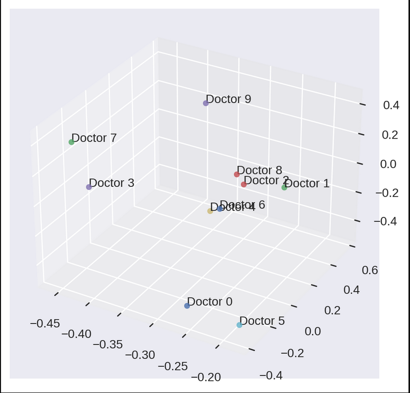
Notice how some docotors are closer to each other while others are far apart. Even if we think every individual has their own choice and are different from each other, we can surely find some patterns in data that can give an idea about the herd behaves. But this not what will help us in recommending channels for doctors. Let's see how we plan to do it. We have to first plot matrix $V$ for that.

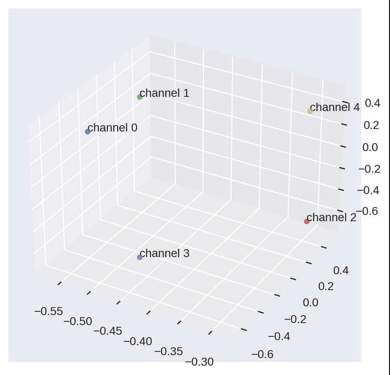
We can see how channels lie in the eigen channel space. This is how a typical doctor thinks about the channels mathematically. Channel 0 and channel 1 are closer to each other, which one can also expect by looking at the vectors of matrix $A$ .

Now that we understand what SVD does for us, its time to make a recommender system.

def recommend(liked_channel, VT, output_num=2):
    global rec
    rec = []
    for item in range(len(VT.columns)):
        if item != liked_channel:
            rec.append([item,np.linalg.norm(Vt[item] - Vt[liked_channel])])
    final_rec = [i[0] for i in sorted(rec, key=lambda x: x[1])]
    return final_rec[:output_num]

This function will give us top two nearest channels in the eigen space based on the euclidean distance.

recommend(1, Vt)
# Output: [4,0]

So, if a doctor likes channel 1, he may also probably like channel 4 and channel 0. This is how we can use SVD for recommendation purpose!!

Uptil now we dealt primarily with singular value decomposition and its application in the context of recommendation systems. Although the system we built in this post is extremely simple, especially in comparison to the complex models that companies use in real-life situations, nonetheless our exploration of SVD is valuable in the sense that we started from the bare basics to build our own model. What is even more fascinating is that many recommendation systems involve singular value decomposition in one way or another, meaning that our exploration is not detached from the context of reality. Hopefully till now I have given you some intuition behind how recommendation systems work and what math is involved in those algorithms. However, the example we used was a dense matrix; meaning, we had all the information about all the doctors. In real world this is not possible, therefore we will have a sparse matrix.

3. Reverse SVD (Sparse matrix)

As we have a good understanding of what SVD is and how it models the ratings, we can get to the heart of the matter: using SVD for for prediction which later can be used for recommendation purpose. Or rather, using SVD for predicting missing ratings. Let $B$ be a ratings matrix, which is made sparse from the original matrix $A$ :

B = A.copy()
B[B < density] = 0  # Introduce sparsity

| | 0 | 1 | 2 | 3 | 4 | | 0 | 0.543405 | 0 | 0.424518 | 0.844776 | 0 | | 1 | 0 | 0.670749 | 0.825853 | 0 | 0.575093 | | 2 | 0.891322 | 0 | 0 | 0 | 0 | | 3 | 0.978624 | 0.811683 | 0 | 0.816225 | 0 | | 4 | 0.431704 | 0.94003 | 0.817649 | 0.336112 | 0 | | 5 | 0.372832 | 0 | 0 | 0.795663 | 0 | | 6 | 0.598843 | 0.603805 | 0 | 0.381943 | 0 | | 7 | 0.890412 | 0.980921 | 0 | 0.890546 | 0.576901 | | 8 | 0.74248 | 0.630184 | 0.581842 | 0 | 0 | | 9 | 0.544685 | 0.769115 | 0 | 0 | 0.852395 |

By sparse, we here mean "with missing entries", not "containing a lot of zeros". Here we convert the missing entries to zero for simple representation.

Oooops

Now guess what: The SVD of $B$ is not defined. It does not exist. Yup, it is impossible to compute, it is not defined, it does not exist :). But don't worry, all your efforts to read this article that far were not futile.

For a dense $B$ we have already calculated its SVD.

But as $B$ is sparse, the matrices $BB^{T}$ and $B^{T}B$ do not exist, so their eigenvectors do not exist either and we can't factorize $B$ as the product $U\Sigma V^{T}$ . However, there is a way around. A first option that was used for some time is to fill the missing entries of $R$ with some simple heuristic, e.g. the mean of the columns (or the rows). Once the matrix is dense, we can compute its SVD using the traditional algorithms. This works OK, but results are usually highly biased. We will rather use another way, based on a minimization problem.

The alternative

Computing the eigenvectors of $BB^{T}$ and $B^{T}B$ is not the only way of computing the SVD of a dense matrix $B$ . We can actually find the matrices $U$ and $V$ if we can find all the vectors $p_u$ and $q_i$ such that (the $p_u$ make up the rows of $U$ and the $q_i$ make up the columns of $V^{T}$ ). At this point we are assuming that $\Sigma$ will already be multiplied with either $U$ or $V$ and we need not care about it:

$b_{ui} = p_u \cdot q_i$ for all $u$ and $i$ ; $b_{ui}$ are elements of $B$ matrix
All the vectors $p_u$ are mutually orthogonal, as well as the vectors $q_i$ .

Finding such vectors $p_u$ and $q_i$ for all doctors and channels can be done by solving the following optimization problem (while respecting the orthogonality constraints):

$\min_{p_u, q_i\\p_u \perp p_v\\ q_i \perp q_j}\sum_{b_{ui} \in R} (b_{ui} - p_u \cdot q_i)^2$

The above one reads as find vectors $p_u$ and $q_i$ that makes the sum minimal. In other words: we're trying to match as well as possible the values $b_{ui}$ with what they are supposed to be: $p_u \cdot q_i$ .

Once we know the values of the vectors $p_u$ and $q_i$ that make this sum minimal (and here the minimum is zero), we can reconstruct $U$ and $V$ and we get our SVD.

So what do we do when $B$ is sparse, i.e. when some ratings are missing from the matrix? Simon Funk's answer is that we should just not give a crap. We still solve the same optimization problem:

$\min_{p_u, q_i}\sum_{b_{ui} \in R} (b_{ui} - p_u \cdot q_i)^2.$

The only difference is that this time, some ratings are missing, i.e. $B$ is incomplete. Note that we are not treating the missing entries as zeros: we are purely and simply ignoring them. Also, we will forget about the orthogonality constraints, because even if they are useful for interpretation purpose, constraining the vectors usually does not help us to obtain more accurate predictions.

Thanks to his solution, Simon Funk ended up in the top 3 of the Netflix Prize for some time. His algorithm was heavily used, studied and improved by the other teams.

The algorithm

It will be very difficult to find the values of the vectors $p_u$ and $q_i$ that make this sum minimal (and the optimal solution may not even be unique). However, there are tons of techniques that can find approximate solutions. We will here use SGD (Stochastic Gradient Descent).

Gradient descent is a very classical technique for finding the (sometimes local) minimum of a function. If you have ever heard of back-propagation for training neural networks, well backprop is just a technique to compute gradients, which are later used for gradient descent. SGD is one of the zillions variants of gradient descent. We won't detail too much how SGD works (there are tons of good resources on the web) but the general pitch is as follows.

When you have a function $f$ with a parameter $\theta$ that looks like this:

$f(\theta) = \sum_k f_k(\theta),$

the SGD procedue minimizes $f$ (i.e. finds the value of $\theta$ such that $f(\theta)$ is as small as possible), with the following steps:

Randomly initialize $\theta$
for a given number of times, repeat:
- for all $k$ $k$ , repeat:
  - compute $\frac{\partial f_k}{\partial \theta}$
  - update $\theta$ with the following rule: $\theta \leftarrow \theta - \alpha \frac{\partial f_k}{\partial \theta},$$, where $$\alpha$$ is the learning rate (a small value).$

In our case, the parameter $\theta$ corresponds to all the vectors $p_u$ and all the vectors $q_i$ (which we will denote by $(p_*, q_*)$ ), and the function $f$ we want to minimize is

f(p_*, q_*) = \sum_{b_{ui} \in B} (b_{ui} - p_u \cdot q_i)^2 =\sum_{b_{ui} \in B} f_{ui}(p_u, q_i),

where $f_{ui}$ is defined by $f_{ui}(p_u, q_i) = (b_{ui} - p_u \cdot q_i)^2$ .

So, in order to apply SGD, what we are looking for is the value of the derivative of $f_{ui}$ with respect to any $p_u$ and any $q_i$ .

The derivative of $f_{ui}$ with respect to a given vector $p_u$ is given by:
$\frac{\partial f_{ui}}{\partial p_u} = \frac{\partial}{\partial p_u} (b_{ui} - p_u \cdot q_i)^2 = - 2 q_i (b_{ui} - p_u \cdot q_i)$
Symmetrically, the derivative of $f_{ui}$ with respect to a given vector $q_i$ is given by:
$\frac{\partial f_{ui}}{\partial q_i} = \frac{\partial}{\partial q_i} (b_{ui} - p_u \cdot q_i)^2 = - 2 p_u (b_{ui} - p_u \cdot q_i)$

Don't be scared, honestly this is highschool-level calculus.

The SGD procedure then becomes:

Randomly initialize all vectors $p_u$ and $q_i$
for a given number of times, repeat:
- for all known ratings $b_{ui}$ $b_{u i}$ , repeat:
  - compute $\frac{\partial f_{ui}}{\partial p_u}$ and $\frac{\partial f_{ui}}{\partial q_i}$ (we just did)
  - update $p_u$ and $q_i$ with the following rule: $p_u \leftarrow p_u + \alpha \cdot q_i (b_{ui} - p_u \cdot q_i)$ , and $q_i \leftarrow q_i + \alpha \cdot p_u (b_{ui} - p_u \cdot q_i)$ . We avoided the multiplicative constant $2$ and merged it into the learning rate $\alpha$ .

Notice how in this algorithm, the different factors in $p_u$ (and $q_i$ ) are all updated at the same time. Funk's original algorithm was a bit different: he actually trained the first factor, then the second, then the third, etc. This gave his algorithm a more SVDesque flavor.

Once all the vectors $p_u$ and $q_i$ have been computed, we can estimate all the ratings we want using the formula:

$\hat{b}_{ui} = p_u \cdot q_i.$

There's a hat on $\hat{b}_{ui}$ to indicate that it's an estimation, not its real value.

First let's create a sparse matrix $B$ from our original matrix $A$

B = A.copy()
B[B < density] = 0  # Introduce sparsity

We will actually ignore the zeros in our heuristic below Without further ado, here is a Python translation of this algorithm:

# Define the rank for approximation
k = 5  # Target rank for approximation

# Initialize matrices for approximation
U_hat = np.random.rand(10, k)
V_hat = np.random.rand(k, 5)

# Stochastic Gradient Descent (SGD) for SVD
learning_rate = 0.01
epochs = 100

for epoch in range(epochs):
    for i in range(m):
        for j in range(n):
            if A[i, j] != 0: #ignore the values
                error = B[i, j] - np.dot(U_hat[i, :], V_hat[:, j])
                # Update U_hat and V_hat using gradient descent
                U_hat[i, :] += learning_rate * (error * V_hat[:, j])
                V_hat[:, j] += learning_rate * (error * U_hat[i, :])

# Compute the approximation
B_hat = np.dot(U_hat, V_hat)

This is the B_hat that we calculated.

| | 0 | 1 | 2 | 3 | 4 | | 0 | 0.365693 | 0.419717 | 0.200663 | 0.483557 | 0.266186 | | 1 | 0.286331 | 0.563663 | 0.847748 | 0.0151053 | 0.336421 | | 2 | 0.55534 | 0.279551 | 0.0697076 | -0.0146382 | -0.0358394 | | 3 | 0.770152 | 0.753652 | 0.0917435 | 0.759947 | 0.379406 | | 4 | 0.660367 | 0.764434 | 0.706477 | 0.171001 | 0.283622 | | 5 | 0.498131 | 0.312743 | -0.154381 | 0.403127 | -0.0266576 | | 6 | 0.677697 | 0.481115 | -0.0497456 | 0.388942 | 0.12996 | | 7 | 0.995571 | 0.902666 | 0.121597 | 0.903261 | 0.376372 | | 8 | 0.602486 | 0.615277 | 0.554362 | 0.20031 | 0.00650232 | | 9 | 0.612328 | 0.582253 | 0.101819 | 0.487711 | 0.356633 |

Now let us see how our algorithm performed by checking the similarity between $B$ and $A$ We will use cosine similarity for this purpose.

vector1 = A.flatten()
vector2 = B_hat.flatten()

# Compute cosine similarity
dot_product = np.dot(vector1, vector2)
norm_vector1 = np.linalg.norm(vector1)
norm_vector2 = np.linalg.norm(vector2)
cosine_similarity = dot_product / (norm_vector1 * norm_vector2)

print("Cosine Similarity between the two matrices:", cosine_similarity)

Output: "Cosine Similarity between the two matrices: 0.9422853785701409"

This means that our matrices are fairly similar and the algorithm works.

4. Conclusion

we dealt primarily with singular value decomposition and its application in the context of recommendation systems. Although the system we built in this post is extremely simple, especially in comparison to the complex models that companies use in real-life situations, nonetheless our exploration of SVD is valuable in that we started from the bare basics to build our own model. What is even more fascinating is that many recommendation systems involve singular value decomposition in one way or another, meaning that our exploration is not detached from the context of reality. Hopefully this post has given you some intuition behind how recommendation systems work and what math is involved in those algorithms. I hope you now understand how beautiful SVD is, and how we can adapt SVD to a recommendation problem.

5. Resources

Work of Nicolas Hug which greatly inspired this post. Amazing lecture by the GOAT Prof. Gilbert Strang. I am highly indebted to his lectures on linear algebra and is always a refresher whenever I watch it again. Here's a shorter version. This video shows the physical signifinace of SVD and how the factorisation is nothing but a rotation followed by scaling followed by rotation again. If you want to calculate the left and right singular vectors by this video might come handy This post by Zachariah Miller serves a great example for understanding recommendation system as a beginner.

Authored by Chirag Patil

1. Understanding SVD

2. SVD for recommendation (Dense matrix)

3. Reverse SVD (Sparse matrix)

Oooops

The alternative

The algorithm

4. Conclusion

5. Resources

More in Data Systems & Applied AI

Top Talent: The OpenAI Database Story

Maximizing the BigQuery Free Tier: A Complete Cost Control Guide

Pandas vs Polars vs DuckDB - Performance Showdown on Flight Data